Stochastic Gradient Descent
19 Jan 2024Gradient descent is a method for unconstrained mathematical optimization. The direction of gradient of a function is in the direction of its maximum. In ML, the idea is to iteratively move in the direction opposite to the gradient, to reach a local minima in the loss landscape. i.e. \(x_{k+1} = x_k - \gamma \nabla F(x)\) \(x_{k+1} = x_k - \gamma \underbrace{\frac{1}{n} \sum_{i=1}^n \nabla f_i(x)}_{\text{over all data points}}\)
Stochastic Gradient Descent speeds this up by replacing the computation over all data points in each iteration to just 1 data point in each iteration.
\(x_{k+1} = x_k - \gamma \underbrace{\nabla f(x)}_{\text{only 1 data point}}\)
The computation is now n times faster.
In a DNN, which creates a non-convex surface, smaller learning rate takes small steps to find the minima.

For a very tiny learning rate (= step size) things are very stable, especially in the beginning.
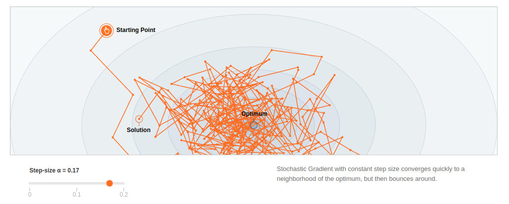
SGD is much more sensitive to learning rate than GD, since the 2nd term in the equation is now a very small contribution. Choice of learning rate is still an open problem.
Things become more chaotic closer to the optimum. So SGD is a good choice in large ML problems where I can reach near optimum fast and I don’t have to reach the optimum because I don’t want to overfit on the data. Lack of exact convergence is explained away for robustness.
Why does SGD behave this way?
Take a simple 1D optimization problem as an example : Least Squares Problem
\(\text{min} f(x) = \frac{1}{2} \sum_{i=1}^n(a_ix-b_i)^2\)
n individual loss functions exist for each data point. Minimum of individual component is
\(\text{minimum of } f_i(x) = \frac{1}{2} (a_ix-b_i)^2 \text{ by equating }f_i(x)\text{ to 0 is } x_i^* = \frac{b_i}{a_i}\)
which gives the lower bound of the optimum. The bounds of the optimum solution will be \(x^* \in \left[ \text{min}_i^* , \text{max}_i^* \right]\)
TBD: Add image showing bounds and far out zone
In the far out zone, \(\text{full gradient is } \nabla f(x)=\sum_i a_i(a_ix-b_i)\) \(\text{stochastic gradient is } \nabla f_i(x)= a_i(a_ix-b_i)\) \(\nabla f_i(x) \text{ has the same sign as } \nabla f(x)\) i.e. even though stochastic gradient is not the full gradient, it has some component in the direction of the full gradient. The stochastic gradient makes an acute angle with the full gradient. So moving in that direction is a good idea, especially in the beginning. By the time you do 1 GD step you can do n SGD steps to move in the correct direction. This is what gives it the dramatic initial progress.
In the region of confusion, this behaviour breaks down. \(\text{Some} \nabla f_i(x) \text{ has the same sign as } \nabla f(x) \text{while some do not}\) giving rise to the fluctuations.
Why does this work?
Stochastic gradient is an unbiased estimate of the true gradient. The key thing controlling the speed of SGD is the variance in the stochastic gradients. The smaller the variance, the better estimate my stochastic gradient is for the true gradient.
Mini-batch Gradient Descent is the best of both worlds, capitalizing on parallel computes on GPU.
\(x_{k+1} = x_k - \frac{\gamma}{b} \underbrace{\sum_{i=1}^b \nabla f_i(x)}_{\text{batch size of b}}\)
Each core can compute 1 stochastic gradient.
Very large mini-batches resemble true GD, shrinks the region of confusion, but is not favourable in DNN because that starts overfitting on test set.
References:
- Wikipedia
- MIT OCW 18.065 Lecture 25: Stochastic Gradient Descent by Suvrit Sra
- Visualization from Fabian Pedregosa’s blog